 Physics Research Project
To finalize my Bachelor in Physics, I had to conduct a research project. For this, I joined the Large Hadron Collider beauty (LHCb) group in Groningen, working with CERN. Below, you may find a summary of the whole project: the problem statement and context, how the analysis was performed, necessary and developed digital competencies and a sample of the results. For a more in depth description and viewing of the code snippets, see the dedicated github repository.
Problem Statement and Context
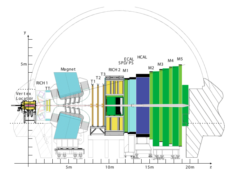
The LHCb group at CERN had recently replaced one of the subdetectors, named Vertex Locator (VELO), for a pixel-based version. These pixels were in charge of signaling a hit when a charged particle would travel through them. In essence, the pixel would measure a hit if the electric current generated by the passing of a charged particle was above a certain threshold. The threshold could not be too large, for it would not detect all of the particles, nor too low, as electric fluctuations within the components would cause false measurements. Thus came the need to calibrate the thresholds of the pixels. The issue I was tasked with spreading light on was on the presence and nature of the heterogeneity between the pixels. Should I find the pixels had a homogeneous response to the travelling particles, these could be calibrated in unison. On the contrary, should there be a heterogeneity between them, they would need to be calibrated individually.
Project Build
- Load the provided data: a large amount of 256x256 csv files, representing the pixel grid and the recorded hits for a number of measurement runs and thresholds.
- Transform the data into flux (hits per second) for each threshold and save the csv files.
- Fit the transformed data (flux per threshold) into a mathematical model for each pixel and the pixel grid as a whole.
- Visualize the results: compare the behaviour of individual pixels against the average one on a scatter plot and showcase the fitted parameters and fit type for each pixel in a heatmap representing the pixel grid. Draw conclusions from these.
- Perfom the proper error analysis through points 2, 3 and 4 and repeat the above steps in a loop to analyze all four sets of data.
Digital Competencies
Specifically for the computational aspect, this project required or taught me, among others, good Python knowledge of,
- file management: loading and saving files and images in different formats,
- NumPy for data analysis and matrix computations,
- SciPy for mathematical modeling and fitting and
- Matplotlib Pyplot for scatter and line plots and colored grids.
Results and Conclusions
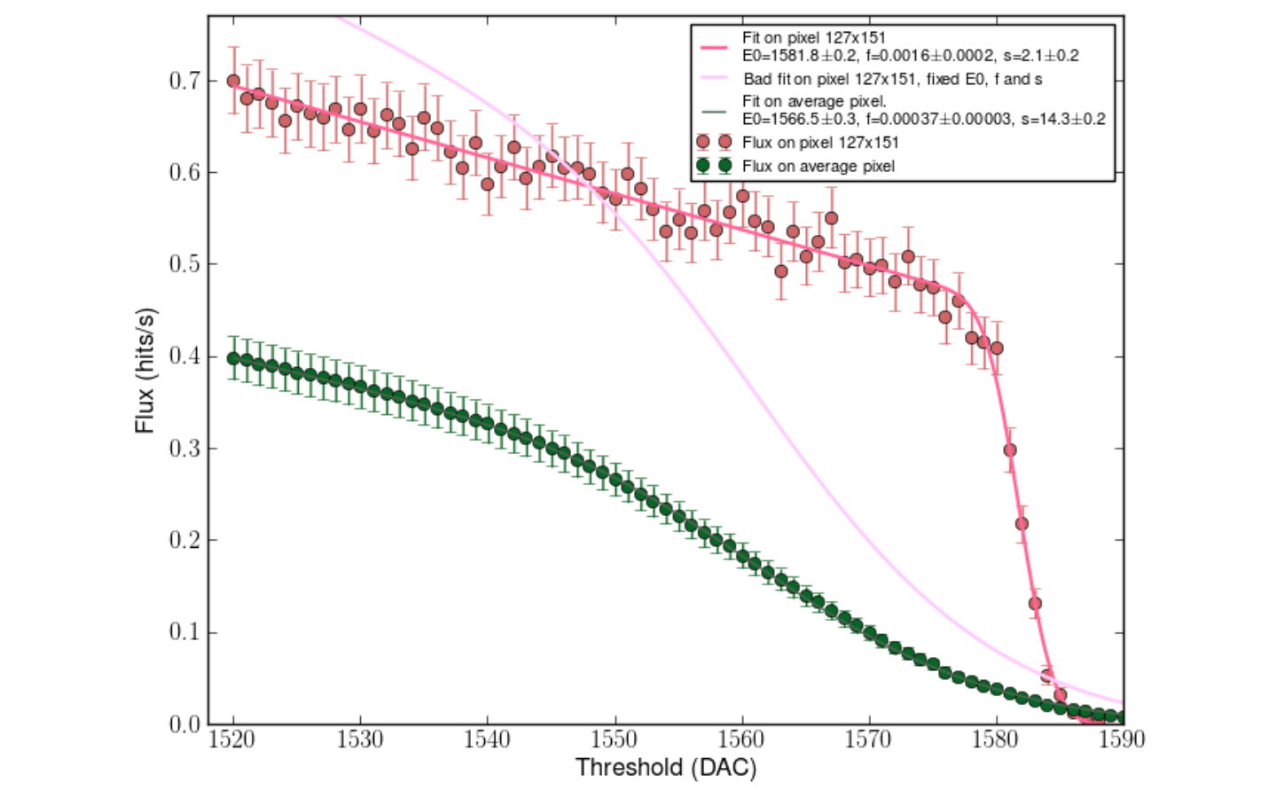 While I will not discuss the project conlcusions itself in detail, I shall showcase here a sample of the obtained results. You may find
on the right a plot showing the flux on an arbitrary pixel and the average pixel, along with their fits. The average pixel has a good fit
with three free parameters, while the individual pixel has a good fit if all three parameters are free. If these are fixed to the results
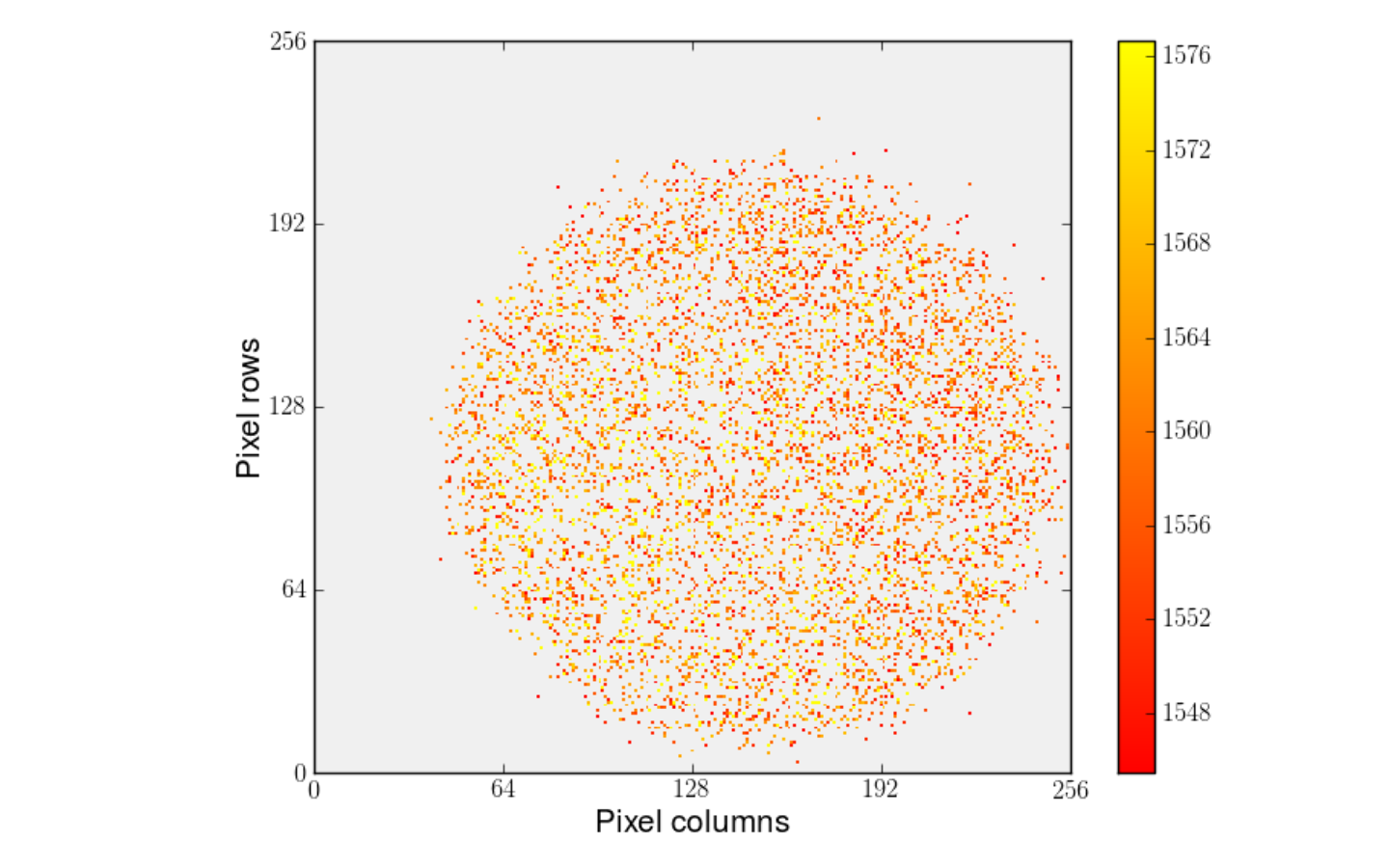
of the average pixel, the resulting fit does not resemble the data points. Below, you may find the heatmaps. The first one shows the value
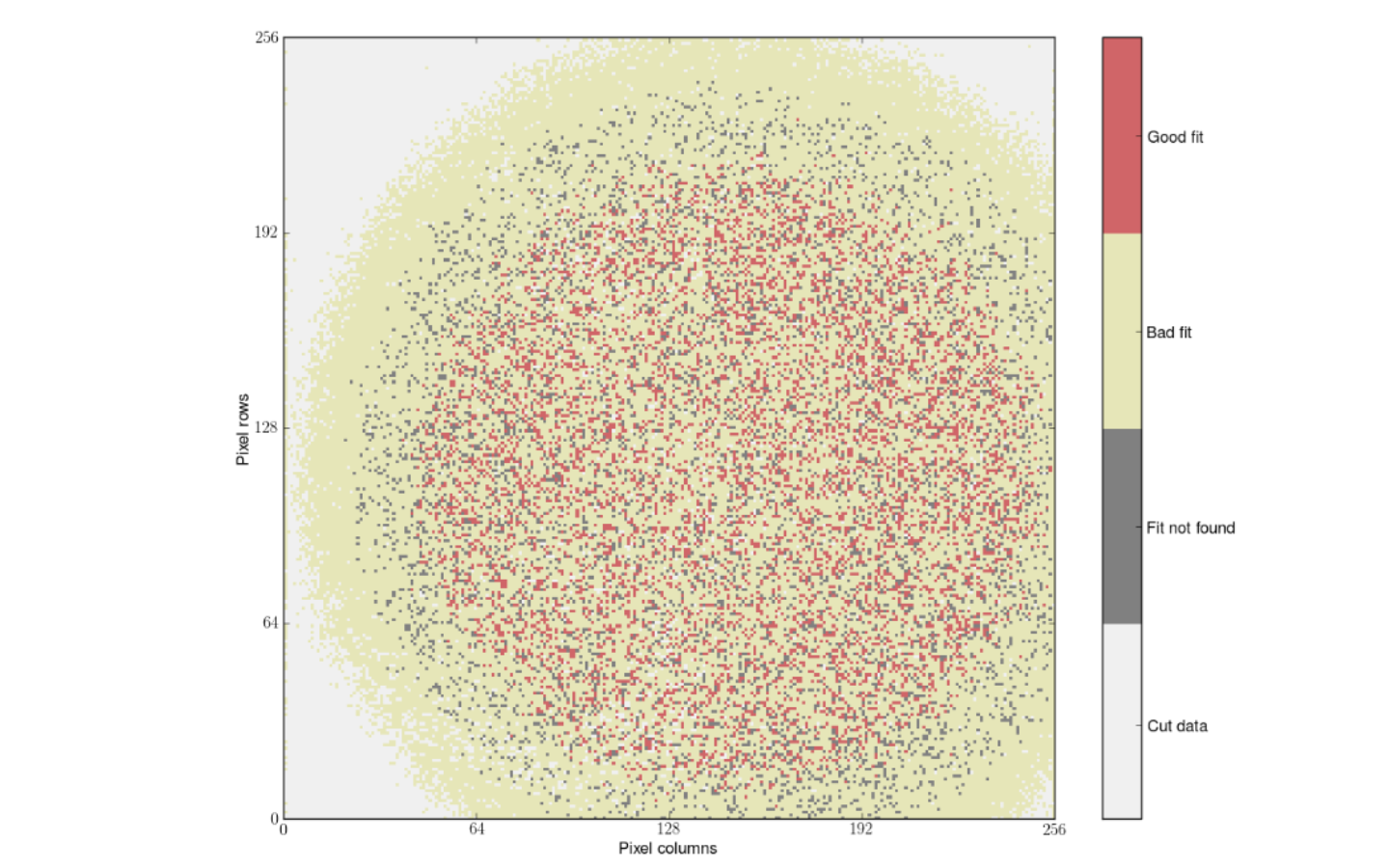
of one of the fitted parameters for each pixel of the grid, where grey represents no fit was attempted or found. The second shows the
arbitrarily defined fit type for each pixel of the grid. Many more figures for each set of data, fitted parameters and some more pixels were
generated, from which conclusions were derived. Perhaps it is already apparent with the figures here presented that some heterogeneity is indeed
present within the pixels and further calibration measurements are thereupon required to individually set the threshold for each pixel. If you
would like to know more about the research project and conclusions or view the thesis, click here.
While I will not discuss the project conlcusions itself in detail, I shall showcase here a sample of the obtained results. You may find
on the right a plot showing the flux on an arbitrary pixel and the average pixel, along with their fits. The average pixel has a good fit
with three free parameters, while the individual pixel has a good fit if all three parameters are free. If these are fixed to the results
of the average pixel, the resulting fit does not resemble the data points. Below, you may find the heatmaps. The first one shows the value
of one of the fitted parameters for each pixel of the grid, where grey represents no fit was attempted or found. The second shows the
arbitrarily defined fit type for each pixel of the grid. Many more figures for each set of data, fitted parameters and some more pixels were
generated, from which conclusions were derived. Perhaps it is already apparent with the figures here presented that some heterogeneity is indeed
present within the pixels and further calibration measurements are thereupon required to individually set the threshold for each pixel. If you
would like to know more about the research project and conclusions or view the thesis, click here.